Solving the Coolest Integral Ever – Fourier Series, Gamma Functions, and the Riemann Zeta Function

Chancellor Ceti

2025-10-18

Table of Contents

Introduction

A few days ago, I was feeling a bit low, so like any normal person, I lay in bed for several hours solving integrals I found on Youtube. I would open a video, pause it at the start, solve the problem, and then see how the uploader had done it. This went on for a long time until I found one Maths505 video that changed the course of my Sunday afternoon. The problem in the video was itself fairly normal, but in the comments section, a certain gentleman by the name of "TiFn4G" suggested an integral for Maths505 to do:

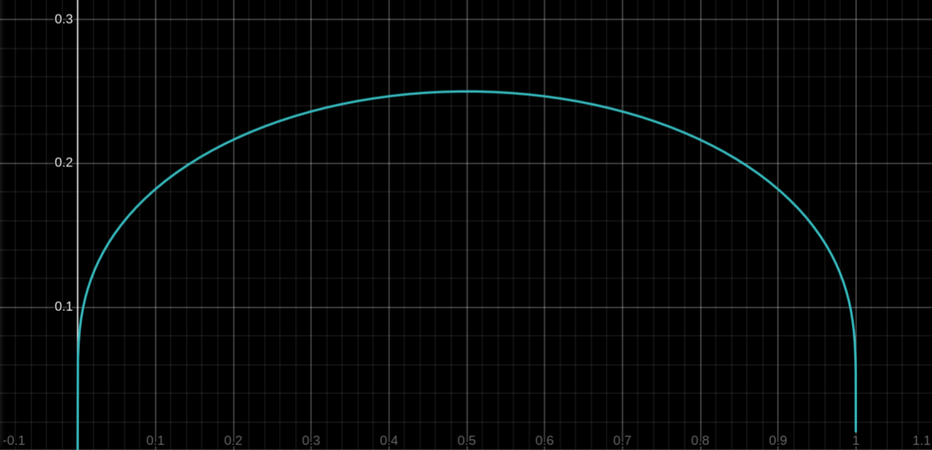
I=\int_{0}^{1}\frac{x-\frac{1}{2}}{\ln(\frac{x}{1-x})}\,dx

Through a lucky find in the comments section, I encountered the love of my life: this integral is the most elegant one I have ever seen. Since I loved the problem so much, I thought I would share the solution with other underemployed people on the internet. I encourage readers to attempt this problem on their own before going to the next section; it’s rare to find a problem this fun, so don’t spoil it by checking the solution before you’ve completely exhausted yourself!

With that out of the way, let’s jump into the actual solution.

Bringing in the gamma function – an observation about the integrand’s structure

The integrand is very gnarly, and the problem presents a definite integral, which led me to believe that no elementary antiderivative exists here. Given this hunch, we already have some clues about what kind of tactics need to be employed here. The first thing that jumped out at me was that the integrand was very similar to \frac{x-1}{\ln x}, which has the convenient integral representation

\int_{0}^{1}x^s\,ds=\frac{x-1}{\ln x}

The function x^s, when multiplied by other terms resulting from our algebraic manipulation, seemed likely to yield some useful properties. So I decided to try breaking up the integrand in a way that would let me use this integral representation.

The logarithm in the denominator is tricky to rearrange, so I decided to instead focus on the numerator and try isolating a term of \frac{x}{1-x} over there.

If we let u=\frac{x}{1-x}, we can find

u-ux=x

x=\frac{u}{u+1}=\frac{u+1-1}{u+1}=1-\frac{1}{u+1}

This yields

x-\frac{1}{2}=\frac{1}{2}-\frac{1}{u+1}=\frac{u+1}{2(u+1)}-\frac{2}{2(u+1)}=\frac{u-1}{2(u+1)}

Note u+1=\frac{x}{1-x}+\frac{1-x}{1-x}=\frac{1}{1-x}

x-\frac{1}{2}=\frac{\frac{x}{1-x}-1}{2/(1-x)}

Therefore,

\frac{x-\frac{1}{2}}{\ln(\frac{x}{1-x})}=(1-x)\frac{\frac{x}{1-x}-1}{2\ln(\frac{x}{1-x})}

I=\int_{0}^{1}\frac{x-\frac{1}{2}}{\ln(\frac{x}{1-x})}=\frac{1}{2}\int_{0}^{1}(1-x)\frac{\frac{x}{1-x}-1}{\ln(\frac{x}{1-x})}

Excellent! Now it becomes clear how we can use the aforementioned integral representation.

I=\frac{1}{2}\int_{0}^{1}(1-x)\left(\int_{0}^{1}\left(\frac{x}{1-x}\right)^s\,ds\right)\,dx=\frac{1}{2}\int_{0}^{1}\left(\int_{0}^{1}x^s(1-x)^{1-s}\,ds\right)\,dx

Since the integrand is measurable and nonnegative for all the values of x and s within the region of integration, Tonelli’s Theorem lets us exchange the order of integration to find

I=\frac{1}{2}\int_{0}^{1}\left(\int_{0}^{1}x^s(1-x)^{1-s}\,dx\right)\,ds

As we had hoped, the integral representation involving x^s did indeed yield a convenient expression. We know that

B(m,n)=\frac{\Gamma(m)\Gamma(n)}{\Gamma(m+n)}=\int_{0}^{1}x^{m-1}(1-x)^{n-1}\,dx

Note that s=(s+1)-1 and (1-s)=(2-s)-1, so that

So our integral now becomes

I=\frac{1}{2}\int_{0}^{1}B(s+1,2-s)\,dx=\frac{1}{2}\int_{0}^{1}\frac{\Gamma(s+1)\Gamma(2-s)}{\Gamma(3)}\,ds

I=\frac{1}{4}\int_{0}^{1}\Gamma(s+1)\Gamma(2-s)\,ds

Again, we’re forced to marvel at the ingenuity of this problem and how nicely everything simplifies. The integrand’s structure now makes the next step obvious: rearranging to utilize the reflection property i.e.

\Gamma(s)\Gamma(1-s)=\frac{\pi}{\sin(\pi s)}

Note that

\Gamma(s+1)\Gamma(2-s)=\biggl(s\Gamma(s)\biggr)\biggl((1-s)\Gamma(1-s)\biggr)=s(1-s)\cdot \Gamma(s)\Gamma(1-s)

So we find that

I=\frac{1}{4}\int_{0}^{1}s(1-s)\cdot \frac{\pi}{\sin(\pi s)}\,ds=\frac{\pi}{4}\int_{0}^{1}\frac{s(1-s)}{\sin(\pi s)}\,ds

There are a few approaches to this. My instinct told me that a contour integral approach could likely work, but a solution using Fourier series seemed more tractable. \frac{\cos(2\pi ns)}{\sin(\pi s)} presents a world of useful properties and recurrence relations. Thus, we arrive at the next chapter of our journey.

Finding the Fourier Series for s(1-s)

This part involves fairly standard calculations, but for completeness and the benefit of less experienced calculus students, I have included all the steps.

We seek a series representation of the form

s(1-s)=\sum_{k=0}^{\infty}a_k\cos(2\pi ks)

By multiplying both sides by \cos(2\pi js) and integrating from 0 to 1, it is easily found that

a_0=\int_{0}^{1}s(1-s)\,ds=\frac{1}{6}

a_k=2 \int_{0}^{1}s(1-s)\cos(2\pi ks)\,ds

This second integral is easily evaluated using integration by parts (details omitted because anyone who’s gotten this far knows how to do it):

a_k=\frac{-u\cos u}{2(\pi k)^3}\Bigg|_{0}^{2\pi k}=\frac{-1}{\pi^2 k^2}

Thus,

s(1-s)=\frac{1}{6}-\frac{1}{\pi^2}\sum_{k=1}^{\infty}\frac{\cos(2\pi ks)}{k^2}

We can substitute this back into our integral to find

I=\frac{\pi}{4}\int_{0}^{1}\csc(\pi s)\left(\frac{1}{6}-\frac{1}{\pi^2}\sum_{k=1}^{\infty}\frac{\cos(2\pi ks)}{k^2}\right)\,ds

I=\frac{\pi}{24}\int_{0}^{1}\csc(\pi s)\,ds-\frac{1}{4\pi}\int_{0}^{1}\left(\sum_{k=1}^{\infty}\frac{\cos(2\pi ks)}{\sin(\pi s)\cdot k^2}\right)\,ds

This looks intimidating, but the magic potato energy of the universe makes it possible to go further.

A Brief Analysis Interlude for the Depraved

The first thing most readers will notice is that \csc(\pi s) has a singularity at s=0, making everything here diverge if we naively go about this. To avoid that problem, truncate the bounds of integration to be [\epsilon,1-\epsilon] where \epsilon \to 0. Once the limit is taken, the integrals will be the same on the truncated bounds as they are on [0,1].

Now, it becomes clear that, at some point, the ability to interchange summation and integration in the right-hand term will be useful. However, the presence of \sin(\pi s) makes it dubious whether that is possible due to issues of divergence. We can demonstrate uniform convergence to prove the validity of interchanging these operators.

Define

S_N(s)=\sum_{k=1}^{N}\frac{\cos(2\pi ks)}{k^2}=\sum_{k=1}^{N}g_k(s)

S(s)=\lim_{N\to \infty}S_N(s)

We find that

\left|g_k(s)\right|=\left|\frac{\cos(2\pi ks)}{k^2}\right|\le\frac{\left|\cos(2\pi ks)\right|}{k^2}\le \frac{1}{k^2}

Now, if we let M_k=\frac{1}{k^2}, we can use the Weierstrass M-test to find

\left|g_k(s)\right|\le M_k

And we see that \sum_{k=1}^{N}M_k converges

\lim_{N\to\infty}\sum_{k=1}^{N}M_k=\sum_{k=1}^{\infty}\frac{1}{k^2}=\zeta(2)=\frac{\pi^2}{6}

Therefore, S_N(s)=\sum_{k=1}^{N}g_k(s) converges absolutely and uniformly i.e.

\lim_{N\to\infty} \sup_{s \in [0,1]}\left|S_N(s)-S(s)\right|=0

Now, our integrand is \csc(\pi s)S_N(s)

Recall that we truncated the bounds of integration to be [\epsilon,1-\epsilon] where \epsilon\to 0. So we seek to prove uniform convergence on that interval.

We find

\left|\csc(\pi s)S_N(s)-\csc(\pi s)S(s)\right| =\csc(\pi s)\left|S_N(s)-S(s)\right|\le\csc(\pi s)\sup_{s \in [\epsilon,1-\epsilon]}\left|S_N(s)-S(s)\right|

As N\to\infty, that final expression goes to zero due to the uniform convergence of S_N(s) – note that [\epsilon,1-\epsilon] is a subset of [0,1], so the uniform convergence of S_N on [0,1] applies on the truncated interval as well.

This yields

\lim_{N\to\infty}\sup_{s\in [\epsilon,1-\epsilon]}\left|\csc(\pi s)S_N(s)-\csc(\pi s)S(s)\right|=0

Therefore, the integrand \sum_{k=1}^{N}\frac{\cos(2\pi ks)}{\sin(\pi s)\cdot k^2} converges uniformly, so we can interchange summation and integration!

Finding a recurrence relation and turning the integral into a more tractable series

With that brief foray into analysis completed, let us return to our problem

I=\frac{\pi}{24}\int_{0}^{1}\csc(\pi s)\,ds-\frac{1}{4\pi}\int_{0}^{1}\left(\sum_{k=1}^{\infty}\frac{\cos(2\pi ks)}{\sin(\pi s)\cdot k^2}\right)\,ds

Having just proved uniform convergence of the sum being integrated, we can interchange summation and integration to get

I=\lim_{\epsilon\to0}\left(\frac{\pi}{24}\int_{\epsilon}^{1-\epsilon}\csc(\pi s)\,ds-\frac{1}{4\pi}\sum_{k=1}^{\infty}\frac{1}{k^2}\left(\int_{\epsilon}^{1-\epsilon}\frac{\cos(2\pi ks)}{\sin(\pi s)}\,ds\right)\right)

Note that we also moved \frac{1}{k^2} out of the integral since it is a constant with respect to s.

This most recent form of the integral suggests a search for a recurrence relation as the most reasonable next step. We know that \cos(2\pi ks)-\cos(2\pi(k-1)s) has a useful formula in terms of sines, so it seems probable that a recurrence relation of some sort can be found for \int_{0}^{1}\frac{\cos(2\pi ks)}{\sin(\pi s)}\,ds.

This approach has the added benefit of offering the possibility of cancelling out the first cosecant integral that diverges.

Before doing that, though, introduce the substitution u=\pi s and get

I=\lim_{\epsilon\to0}\left(\frac{1}{24}\int_{\epsilon}^{\pi(1-\epsilon)}\csc(u)\,du-\frac{1}{4\pi^2}\sum_{n=1}^{\infty}\frac{1}{n^2}\left(\int_{\epsilon}^{\pi(1-\epsilon)}\frac{\cos(2nu)}{\sin(u)}\,du\right)\right)

With that done, we’re ready to look for our recurrence relation. Define

L_n(\epsilon)=\int_{\epsilon}^{\pi(1-\epsilon)}\frac{\cos(2nu)}{\sin(u)}\,du

Now recall the trigonometric identity

\cos\alpha-\cos\beta=-2\sin\left(\frac{\alpha+\beta}{2}\right)\sin\left(\frac{\alpha-\beta}{2}\right)

Using this, we find that

L_{n-1}(\epsilon)-L_n(\epsilon)=-2 \int_{\epsilon}^{\pi(1-\epsilon)}\frac{\sin((2n-1)x)\sin(-x)}{\sin x}\,dx =2 \int_{\epsilon}^{\pi(1-\epsilon)}\sin((2n-1)x)\,dx

Note that this integral no longer has any singularities, so we can safely take the limit

\lim_{\epsilon\to0}\left(L_{n-1}(\epsilon)-L_n(\epsilon)\right)=2 \int_{0}^{\pi}\sin((2n-1)x)\,dx

\lim_{\epsilon\to0}\left(L_{n-1}(\epsilon)-L_n(\epsilon)\right)=\frac{-2}{2n-1}\cos x\Big|_{0}^{2\pi n-\pi}=\frac{4}{2n-1}

We can sum over this relation from 1 to n to find

\lim_{\epsilon\to0}\left(\sum_{k=1}^{n}\left(L_{k-1}(\epsilon)-L_k(\epsilon)\right)\right)=\sum_{k=1}^{n}\frac{4}{2k-1}

Alo notice that this sum telescopes, i.e.

\lim_{\epsilon\to0}\left(\sum_{k=1}^{n}(L_{k-1}(\epsilon)-L_k(\epsilon))\right)=\lim_{\epsilon\to0}\left(-L_n(\epsilon)+L_0(\epsilon)\right)

Therefore,

\lim_{\epsilon\to0}\left(L_0(\epsilon)-L_n(\epsilon)\right)=\sum_{k=1}^{n}\frac{4}{2k-1}

\lim_{\epsilon\to0}L_n(\epsilon)=\lim_{\epsilon\to0}\left(L_0(\epsilon)-\sum_{k=1}^{n}\frac{4}{2k-1}\right)=\lim_{\epsilon\to0}\left(L_0-\sum_{k=0}^{n-1}\frac{4}{2k+1}\right)

Now recall that, with our limiting procedure involving \epsilon,

I=\lim_{\epsilon\to0}\left(\frac{1}{24}\int_{\epsilon}^{\pi(1-\epsilon)}\csc(u)\,du-\frac{1}{4\pi^2}\sum_{n=1}^{\infty}\frac{1}{n^2}\left(\int_{\epsilon}^{\epsilon(1-\pi)}\frac{\cos(2nu)}{\sin(u)}\,du\right)\right)

=\lim_{\epsilon\to0}\left(\frac{1}{24}\int_{\epsilon}^{\pi(1-\epsilon)}\csc(u)\,du-\frac{1}{4\pi^2}\sum_{n=1}^{\infty}\frac{1}{n^2}L_n(\epsilon)\right)

=\lim_{\epsilon\to0}\left(\frac{1}{24}\int_{\epsilon}^{\pi(1-\epsilon)}\csc(u)\,du-\frac{1}{4\pi^2}\sum_{n=1}^{\infty}\frac{1}{n^2}\left(L_0(\epsilon)-\sum_{k=0}^{n-1}\frac{4}{2k+1}\right)\right)

=\lim_{\epsilon\to0}\left(\frac{1}{24}\int_{\epsilon}^{\pi(1-\epsilon)}\csc(u)\,du-\frac{1}{4\pi^2}L_0(\epsilon)\zeta(2)+\frac{1}{\pi^2}\sum_{n=1}^{\infty}\frac{1}{n^2}\sum_{k=0}^{n-1}\frac{1}{2k+1}\right)

Now, the observant reader will notice that

\lim_{\epsilon\to0}\int_{\epsilon}^{\pi(1-\epsilon)}\csc u\,du=\lim_{\epsilon\to 0}\int_{\epsilon}^{\pi(1-\epsilon)}\frac{\cos(2u\cdot 0)}{\sin u}\,du=\lim_{\epsilon\to0}L_0(\epsilon)

Therefore,

\lim_{\epsilon\to0}\left(\frac{1}{24}\int_{\epsilon}^{\pi(1-\epsilon)}\csc(u)\,du-\frac{1}{4\pi^2}L_0(\epsilon)\zeta(2)\right) =\lim_{\epsilon\to0}\left(\frac{L_0(\epsilon)}{24}-L_0(\epsilon)\cdot\left(\frac{1}{4\pi^2}\right)\left(\frac{\pi^2}{6}\right)\right) =\lim_{\epsilon\to0}L_0(\epsilon)\left(\frac{1}{24}-\frac{1}{24}\right)=0

Excellent cancellation of the divergent terms! We are left with

I=\lim_{\epsilon\to0}\left(\frac{1}{\pi^2}\sum_{n=1}^{\infty}\frac{1}{n^2}\sum_{k=0}^{n-1}\frac{1}{2k+1}\right)

Note that no terms involving \epsilon are left, so we can remove the limit and get

I=\frac{1}{\pi^2}\sum_{n=1}^{\infty}\frac{1}{n^2}\sum_{k=0}^{n-1}\frac{1}{2k+1}

Now notice that

\sum_{k=0}^{n-1}\frac{1}{2k+1}=1+\frac{1}{3}+\ldots+\frac{1}{2n-1}=H_{2n}-\sum_{k=1}^{n}\frac{1}{2n}=H_{2n}-\frac{H_n}{2}

where H_n is the n’th harmonic number.

This lets us simplify our series into

I=\frac{1}{\pi^2}\sum_{n=1}^{\infty}\frac{1}{n^2}\left(H_{2n}-\frac{H_n}{2}\right)

We must now evaluate these two sums separately

I=\frac{1}{\pi^2}S_1-\frac{1}{2\pi^2}S_2

S_1=\sum_{n=1}^{\infty}\frac{H_{2n}}{n^2}

S_2=\sum_{n=1}^{\infty}\frac{H_n}{n^2}

Let us begin with the second sum, which has a simpler H_n rather than H_{2n}

A moderately gnarly series

We are considering

S_2=\sum_{n=1}^{\infty}\frac{H_n}{n^2}

The first trick we employ is introducing an integral representation for the harmonic numbers,

H_n=\int_{0}^{1}\frac{1-x^n}{1-x}\,dx

Plugging this in yields

S_2=\sum_{n=1}^{\infty}\frac{1}{n^2}\left(\int_{0}^{1}\frac{1-x^n}{1-x}\,dx\right)=\int_{0}^{1}\frac{1}{1-x}\left(\sum_{n=1}^{\infty}\frac{1-x^n}{n^2}\right)\,dx

The interchange of integration and summation can be justified by Tonelli’s theorem, since \frac{1-x^n}{n^2(1-x)} is measurable and nonnegative for x\in (0,1).

We can use use the definition of the polylogarithm to turn this into a friendlier expression

\mathrm{Li}_n(x)=\sum_{k=1}^{\infty}\frac{x^k}{k^n}

S_2=\int_{0}^{1}\frac{\zeta(2)-\mathrm{Li}_2(x)}{1-x}

Now we must find the integral of \frac{\mathrm{Li}_2(x)}{1-x}.

Apply integration by parts with u=\mathrm{Li}_2(x) and \,dv=\frac{1}{1-x}. We easily find that v=-\ln(1-x)

From the definition of the polylogarithm, we find

\frac{\,d}{\,dx}\mathrm{Li}_n(x)=\sum_{k=1}^{\infty}\frac{kx^{k-1}}{k^n}=\frac{1}{x}\sum_{k=1}^{\infty}\frac{x^k}{k^{n-1}}=\frac{\mathrm{Li}_{n-1}(x)}{x}

So \,du=\frac{\mathrm{Li}_1(x)}{x}

However, note that

\mathrm{Li}_1(x)=\sum_{k=1}^{\infty}\frac{x^k}{k}=-\ln(1-x)

Therefore, \,du=\frac{-\ln(1-x)}{x}

Thus,

\int \frac{\mathrm{Li}_2(x)}{1-x}\,dx=-\ln(1-x)\mathrm{Li}_2(x)-\int \frac{\ln^2(1-x)}{x}\,dx

This new integral can be solved with the substitution t=1-x, yielding

\int \frac{\ln^2(1-x)}{x}\,dx=-\int \frac{ln^2(t)}{1-t}\,dt

Again apply integration by parts with u=\ln^2(t), \,dv=\frac{1}{1-t}, \,du=\frac{2\ln(t)}{t}, v=-\ln(1-t) and find

\int \frac{ln^2(t)}{1-t}\,dt=-\ln^2(t)\ln(1-t)+2\int \frac{\ln(t)\ln(1-t)}{t}\,dt

Finally, apply integration by parts just once more with u=\ln(t) and \,dv=\frac{\ln(1-t)}{t}. Remember the formula for the derivative of \mathrm{Li}_2(x)=\frac{-\ln(1-x)}{x} so v=-\mathrm{Li}_2(t). Thus,

\int \frac{\ln(t)\ln(1-t)}{t}\,dt=-\ln(t)\mathrm{Li}_2(t)+\int \frac{\mathrm{Li}_2(t)}{t}\,dt=-\ln(t)\mathrm{Li}_2(t)+\mathrm{Li}_3(t)

Now go back to our original integral and remember to change t to 1-x everywhere, in accordance with our substitution

\int \frac{\mathrm{Li}_2(x)}{1-x}\,dx=-\ln(1-x)\mathrm{Li}_2(x)-\int \frac{\ln^2(1-x)}{x}\,dx

=-\ln(1-x)\mathrm{Li}_2(x)+\int \frac{\ln^2(t)}{1-t}\,dx

=-\ln(1-x)\mathrm{Li}_2(x)-\ln^2(1-x)\ln(x)-2\ln(1-x)\mathrm{Li}_2(1-x)+2\mathrm{Li}_3(1-x)

Excellent!

Now let’s go back to our earlier expression

S_2=\int_{0}^{1}\frac{\zeta(2)-\mathrm{Li}_2(x)}{1-x}

\begin{gathered} S_2 = \biggl(-\zeta(2)\ln(1-x)+\ln(1-x)\mathrm{Li}_2(x)+\ln^2(1-x)\ln x\\ \qquad+2\ln(1-x)\mathrm{Li}_2(1-x)-2\mathrm{Li}_3(1-x)\biggr)\Big|_{0}^{1} \end{gathered}

Note that \mathrm{Li}_n(0)=0, \mathrm{Li}_n(1)=\sum_{k=1}^{\infty}\frac{1}{k^n}=\zeta(n), and \ln(1)=0. This makes most of the terms go to zero and yields

\sum_{n=1}^{\infty}\frac{H_n}{n^2}=-\zeta(2)ln(0)+\ln(0)\zeta(2)+2\zeta(3)=2\zeta(3)

What an incredible simplification! Now let’s see how to go about the more complicated sum S_1.

A very gnarly series made easier by our having solved a moderately gnarly one

Now for the most intimidating series yet,

S_1=\sum_{n=1}^{\infty}\frac{H_{2n}}{n^2}

Begin by noting that

H_{2n}=\sum_{k=1}^{n}\frac{1}{k}+\sum_{k=n+1}^{2n}\frac{1}{k}=H_n+\sum_{k=1}^{n}\frac{1}{n+k}

Therefore,

S_1=\sum_{n=1}^{\infty}\frac{H_{2n}}{n^2}=\sum_{n=1}^{\infty}\frac{H_n}{n^2}+\sum_{n=1}^{\infty}\sum_{k=1}^{n}\frac{1}{n^2(n+k)}

S_1=2\zeta(3)+\sum_{n=1}^{\infty}\sum_{k=1}^{n}\frac{1}{n^2(n+k)}

This double summation looks intimidating but actually becomes amazingly simple once a partial fraction decomposition is introduced that leads to a telescoping property. We use

\frac{1}{n^2(n+k)}=\frac{1}{n^2k}+\frac{1}{k^2}\left(\frac{1}{n+k}-\frac{1}{n}\right)

This leads to

\begin{aligned} \sum_{n=1}^{\infty}\sum_{k=1}^{n}\frac{1}{n^2(n+k)}&=\sum_{n=1}^{\infty}\frac{1}{n^2}\sum_{k=1}^{n}\frac{1}{k}+\sum_{n=1}^{\infty}\sum_{k=1}^{n}\frac{1}{k^2}\left(\frac{1}{n+k}-\frac{1}{n}\right)\\ &=\sum_{n=1}^{\infty}\frac{H_n}{n^2}+\sum_{n=1}^{\infty}\sum_{k=1}^{n}\frac{1}{k^2}\left(\frac{1}{n+k}-\frac{1}{n}\right)\\ &=2\zeta(3)+\sum_{n=1}^{\infty}\sum_{k=1}^{n}\frac{1}{k^2}\left(\frac{1}{n+k}-\frac{1}{n}\right) \end{aligned}

Now we make a series of maneuvers to try to find a telescoping relation. First notice that we would infinitely prefer to have \frac{1}{n^2} rather than \frac{1}{k^2} so that we can get nice relations to the Riemann zeta function. Therefore, we need to try re-indexing to get that term.

We can re-index using the following argument. Suppose f(k)=\frac{1}{k^2} and g(n,k)=\frac{1}{n+k}-\frac{1}{n}

Then we have a double sum of the form

\begin{aligned} \sum_{n=1}^{\infty}\sum_{k=1}^{n} f(k)g(n,k) &= f(1)g(1,1) \\ &\quad + \bigl[f(1)g(2,1) + f(2)g(2,2)\bigr] \\ &\quad + \bigl[f(1)g(3,1) + f(2)g(3,2) + f(3)g(3,3)\bigr] + \cdots \\ \\ &=f(1)g(1,1)+f(2)\biggl(g(2,2)+g(3,2)+\cdots\biggr) \\ &\quad + f(3)\biggl(g(3,3)+g(4,3)+\cdots\biggr)+\cdots \\ \\ &=\sum_{n=1}^{\infty}f(n)\sum_{k=n}^{\infty}g(k,n) \end{aligned}

So, with our choice of f(k) and g(n,k), we find

\sum_{n=1}^{\infty}\sum_{k=1}^{n}\frac{1}{k^2}\left(\frac{1}{n+k}-\frac{1}{n}\right)=\sum_{n=1}^{\infty}\frac{1}{n^2}\sum_{k=n}^{\infty}\left(\frac{1}{n+k}-\frac{1}{k}\right)

Great, we’ve gotten that \frac{1}{n^2} that leads to zeta function terms, and we also have an inner sum that easily yields a telescoping relation.

Let’s consider the inner sum on its own \begin{split} & \lim_{N\to\infty}\sum_{k=n}^{N}\left(\frac{1}{n+k}-\frac{1}{k}\right) \\ & =\lim_{N\to\infty}\left(\sum_{k=n}^{N-n}\frac{1}{n+k}+\sum_{k=N-n+1}^{N}\frac{1}{n+k}-\sum_{k=n}^{2n-1}\frac{1}{k}-\sum_{k=2n}^{N}\frac{1}{k}\right) \\ & = \lim_{N\to\infty}\left(\sum_{k=n}^{N-n}\frac{1}{n+k}+\sum_{k=N-n+1}^{N}\frac{1}{n+k}-\sum_{k=n}^{2n-1}\frac{1}{k}-\sum_{k=n}^{N-n}\frac{1}{n+k}\right)\\ & = \lim_{N\to\infty}\left(\sum_{k=N-n+1}^{N}\frac{1}{n+k}-\sum_{k=n}^{2n-1}\frac{1}{k}\right)\\ &=-\sum_{k=n}^{2n-1}\frac{1}{k}=-(H_{2n-1}-H_{n-1})=H_{n-1}-H_{2n-1}\\ &=H_n-\frac{1}{n}-\left(H_{2n}-\frac{1}{2n}\right)=H_n-H_{2n}-\frac{1}{2n} \end{split}

Therefore,

\sum_{n=1}^{\infty}\frac{1}{n^2}\sum_{k=n}^{\infty}\left(\frac{1}{n+k}-\frac{1}{k}\right)=\sum_{n=1}^{\infty}\frac{H_n}{n^2}-\sum_{n=1}^{\infty}\frac{H_{2n}}{n^2}-\frac{1}{2}\sum_{n=1}^{\infty}\frac{1}{n^3} =2\zeta(3)-S_1-\frac{\zeta(3)}{2} =\frac{3\zeta(3)}{2}-S_1

Now combine our last few major results to find

\begin{split} S_1 &=2\zeta(3)+\sum_{n=1}^{\infty}\sum_{k=1}^{n}\frac{1}{n^2(n+k)}\\ &=2\zeta(3)+\left(2\zeta(3)+\sum_{n=1}^{\infty}\sum_{k=1}^{n}\frac{1}{k^2}\left(\frac{1}{n+k}-\frac{1}{n}\right)\right)\\ &=4\zeta(3)+\sum_{n=1}^{\infty}\frac{1}{n^2}\sum_{k=n}^{\infty}\left(\frac{1}{n+k}-\frac{1}{n}\right)\\ &=4\zeta(3)+\left(\frac{3\zeta(3)}{2}-S_1\right) \end{split}

And finally, we arrive at

S_1=\sum_{n=1}^{\infty}\frac{H_{2n}}{n^2}=\frac{11\zeta(3)}{4}

Yet another mind-blowing simplification. Now let’s plug our values for S_1 and S_2 into our expression for I to actually solve the integral.

Wrapping up and solving the integral

Our last expression for I was

I=\int_{0}^{1}\frac{x-\frac{1}{2}}{\ln\left(\frac{x}{1-x}\right)}\,dx=\frac{1}{\pi^2}S_1-\frac{1}{2\pi^2}S_2

We found that S_1=\frac{11\zeta(3)}{4} and S_2=2\zeta(3)

Therefore,

\int_{0}^{1}\frac{x-\frac{1}{2}}{\ln\left(\frac{x}{1-x}\right)}\,dx=\frac{11\zeta(3)}{4\pi^2}-\frac{4\zeta(3)}{4\pi^2}=\frac{7\zeta(3)}{4\pi^2}

What an incredible result! We’ve managed to get an answer involving both \pi^2 and \zeta(3), which is really cool.

After having done so much work, it’s easy to lose sight of just how convoluted this process was and how many times the integral proved to have really nice properties that made life easier. Divergent terms appeared several times, such as \int_{0}^{1}\csc(\pi s)\,ds and \lim_{x\to0}\ln(x)\zeta(2), but always in such a manner that they cancelled out and didn’t cause problems, which strikes me as incredible. In the sums, we found lots of recurrence relations and telescoping relations that led to crazy simplifications where almost all the terms disappeared. And we got to introduce all kinds of exotic functions with amazing properties, which further added to the fun – \zeta(s),\Gamma(s), and \mathrm{ Li}_n(x). The vast array of techniques used and the elegance of the solution have made this made my favorite integral and hopefully at least top 10 for my readers as well.

Today we have learnt that the Maths505 comments section may or may not contain the key to enlightenment in the form of indefinite integrals. Hopefully the reader has enjoyed this mathematical nirvana as much as I have. If you have comments, corrections, or random thoughts, feel free to message me on Discord or email me (contact info in the About section of this site). Thanks for reading!